Computing

Computing is any goal-oriented activity requiring, benefiting from, or creating computers. For example, computing includes designing, developing and building hardware and software systems; processing, structuring, and managing various kinds of information; doing scientific research on and with computers; making computer systems behave intelligently; and creating and using communications and entertainment media. Sub-disciplines of computing include computer engineering, software engineering, computer science, information systems, and information technology.

The history of computing is longer than the history of computing hardware and modern computing technology and includes the history of methods intended for pen and paper or for chalk and slate, with or without the aid of tables.

Computing is intimately tied to the representation of numbers. But long before abstractions like the number arose, there were mathematical concepts to serve the purposes of civilization. These concepts include one-to-one correspondence (the basis of counting), comparison to a standard (used for measurement), and the 3-4-5 right triangle (a device for assuring a right angle).

The earliest known tool for use in computation was the abacus, and it was thought to have been invented in Babylon circa 2400 BC. Its original style of usage was by lines drawn in sand with pebbles. Abaci, of a more modern design, are still used as calculation tools today. This was the first known computer and most advanced system of calculation known to date - preceding Greek methods by 2,000 years.

Read More...

Matrices

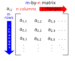
In mathematics, a matrix (plural matrices) is a rectangular array of numbers, symbols, or expressions, arranged in rows and columns. The individual items in a matrix are called its elements or entries. An example of a matrix with 2 rows and 3 columns is

Matrices of the same size can be added or subtracted element by element. But the rule for matrix multiplication is that two matrices can be multiplied only when the number of columns in the first equals the number of rows in the second. A major application of matrices is to represent linear transformations, that is, generalizations of linear functions such as f(x) = 4x. For example, the rotation of vectors in three dimensional space is a linear transformation. If R is a rotation matrix and v is a column vector (a matrix with only one column) describing the position of a point in space, the product Rv is a column vector describing the position of that point after a rotation. The product of two matrices is a matrix that represents the composition of two linear transformations. Another application of matrices is in the solution of a system of linear equations. If the matrix is square, it is possible to deduce some of its properties by computing its determinant. For example, a square matrix has an inverse if and only if its determinant is not zero. Eigenvalues and eigenvectors provide insight into the geometry of linear transformations.

Applications of matrices are found in most scientific fields. In every branch of physics, including classical mechanics, optics, electromagnetism, quantum mechanics, and quantum electrodynamics, they are used to study physical phenomena, such as the motion of rigid bodies. In computer graphics, they are used to project a 3-dimensional image onto a 2-dimensional screen. In probability theory and statistics, stochastic matrices are used to describe sets of probabilities; for instance, they are used within the PageRank algorithm that ranks the pages in a Google search. Matrix calculus generalizes classical analytical notions such as derivatives and exponentials to higher dimensions.

A major branch of numerical analysis is devoted to the development of efficient algorithms for matrix computations, a subject that is centuries old and is today an expanding area of research. Matrix decomposition methods simplify computations, both theoretically and practically. Algorithms that are tailored to particular matrix structures, such as sparse matrices and near-diagonal matrices, expedite computations in finite element method and other computations. Infinite matrices occur in planetary theory and in atomic theory. A simple example of an infinite matrix is the matrix representing the derivative operator, which acts on the Taylor series of a function.

Read More...

Statistics

Statistics is the study of the collection, organization, analysis, interpretation and presentation of data. It deals with all aspects of data, including the planning of data collection in terms of the design of surveys and experiments.

The word statistics, when referring to the scientific discipline, is singular, as in "Statistics is an art." This should not be confused with the word statistic, referring to a quantity (such as mean or median) calculated from a set of data, whose plural is statistics ("this statistic seems wrong" or "these statistics are misleading").

Statistics is alternately described as a mathematical body of science that pertains to the collection, analysis, interpretation or explanation, and presentation of data, or as a branch of mathematics concerned with collecting and interpreting data. Because of its empirical roots and its focus on applications, statistics is typically considered a distinct mathematical science rather than as a branch of mathematics. Some tasks a statistician may involve are less mathematical; for example, ensuring that data collection is undertaken in a way that produces valid conclusions, coding data, or reporting results in ways comprehensible to those who must use them.

Statisticians improve data quality by developing specific experiment designs and survey samples. Statistics itself also provides tools for prediction and forecasting the use of data and statistical models. Statistics is applicable to a wide variety of academic disciplines, including natural and social sciences, government, and business. Statistical consultants can help organizations and companies that don't have in-house expertise relevant to their particular questions.

Statistical methods can summarize or describe a collection of data. This is called descriptive statistics. This is particularly useful in communicating the results of experiments and research. In addition, data patterns may be modeled in a way that accounts for randomness and uncertainty in the observations.

These models can be used to draw inferences about the process or population under study—a practice called inferential statistics. Inference is a vital element of scientific advance, since it provides a way to draw conclusions from data that are subject to random variation. To prove the propositions being investigated further, the conclusions are tested as well, as part of the scientific method. Descriptive statistics and analysis of the new data tend to provide more information as to the truth of the proposition.

"Applied statistics" comprises descriptive statistics and the application of inferential statistics.[verification needed] Theoretical statistics concerns both the logical arguments underlying justification of approaches to statistical inference, as well encompassing mathematical statistics. Mathematical statistics includes not only the manipulation of probability distributions necessary for deriving results related to methods of estimation and inference, but also various aspects of computational statistics and the design of experiments.

Statistics is closely related to probability theory, with which it is often grouped. The difference is, roughly, that probability theory starts from the given parameters of a total population to deduce probabilities that pertain to samples. Statistical inference, however, moves in the opposite direction—inductively inferring from samples to the parameters of a larger or total population. Statistics has many ties to machine learning and data mining.

Read More...

Trigonometry

Trigonometry' (from Greek trigōnon ``triangle + metron ``measure) is a branch of mathematics that studies the relationship of lengths and angles in triangles. The field emerged during the third century BC, evolving out of a understanding of geometry then being used extensively for astronomical studies .

The 3rd century astronomers first noted that the lengths of the sides of a right angle triangle and the angles between those sides have fixed relationships: that is, if at least the length of one side and the value of one angle is known all other angles and lengths can be determined algorithmically. These calculations soon came to be defined as the trigonometric functions and today are pervasive in both pure and applied mathematics: fundamental methods of analysis such as the Fourier Transform, for example, or the wave equation, use trigonometric functions to understand cyclical phenomena across a great many applications in fields as diverse as physics, mechanical and electrical engineering, music and acoustics, astronomy, ecology and biology. Trigonometry is also the foundation of the practical art of surveying.

Trigonometry is most simply associated with planar right angle triangles (a two dimensional triangle with one angle equal to 90 degrees). The applicability to non-right angle triangles exists but, since any non-right angle triangle (on a flat plane) can be bisected to create two right angle triangles, most problems can be reduced to calculations on right angle triangles. Thus the majority of applications relates to right angle triangles. One exceptions to this is Spherical trigonometry, the study of triangles on spheres, surfaces of constant positive curvature, in elliptic geometry (a fundamental part of astronomy and navigation). Trigonometry on surfaces of negative curvature is part of hyperbolic geometry.

Trigonometry basics are often taught in school either as a separate course or as part of a precalculus course.

If one angle of a triangle is 90 degrees and one of the other angles is known, the third is thereby fixed, because the three angles of any triangle add up to 180 degrees. The two acute angles therefore add up to 90 degrees: they are complementary angles. The shape of a triangle is completely determined, except for similarity, by the angles. Once the angles are known, the ratios of the sides are determined, regardless of the overall size of the triangle. If the length of one of the sides is known, the other two are determined. These ratios are given by the following trigonometric functions of the known angle A, where a, b and c refer to the lengths of the sides in the accompanying figure:

Read More...

Analytical Geometry

Analytic geometry, or analytical geometry, has two different meanings in mathematics. The modern and advanced meaning refers to the geometry of analytic varieties. This article focuses on the classical and elementary meaning.

In classical mathematics, analytic geometry, also known as coordinate geometry, or Cartesian geometry, is

the study of geometry using a coordinate system and the principles of algebra and analysis. This contrasts with the synthetic approach of Euclidean geometry, which treats certain geometric notions as primitive, and uses deductive reasoning based on axioms and theorems to derive truth. Analytic geometry is widely used in physics and engineering, and is the foundation of most modern fields of geometry, including algebraic, differential, discrete, and computational geometry.

Usually the Cartesian coordinate system is applied to manipulate equations for planes, straight lines, and squares, often in two and sometimes in three dimensions. Geometrically, one studies the Euclidean plane (2 dimensions) and Euclidean space (3 dimensions). As taught in school books, analytic geometry can be explained more simply: it is concerned with defining and representing geometrical shapes in a numerical way and extracting numerical information from shapes' numerical definitions and representations. The numerical output, however, might also be a vector or a shape. That the algebra of the real numbers can be employed to yield results about the linear continuum of geometry relies on the Cantor–Dedekind axiom.

Co-Ordinates:

In analytic geometry, the plane is given a coordinate system, by which every point has a pair of real number coordinates. The most common coordinate system to use is the Cartesian coordinate system, where each point has an x-coordinate representing its horizontal position, and a y-coordinate representing its vertical position. These are typically written as an ordered pair (x, y). This system can also be used for three-dimensional geometry, where every point in Euclidean space is represented by an ordered triple of coordinates (x, y, z).

Other coordinate systems are possible. On the plane the most common alternative is polar coordinates, where every point is represented by its radius r from the origin and its angle θ. In three dimensions, common alternative coordinate systems include cylindrical coordinates and spherical coordinates.

Read More...

Geomentry

Geometry (Ancient Greek; geo- "earth", -metron "measurement") is a branch of mathematics concerned



with questions of shape, size, relative position of figures, and the properties of space. A mathematician who works in the field of geometry is called a geometer. Geometry arose independently in a number of early cultures as a body of practical knowledge concerning lengths, areas, and volumes, with elements of a formal mathematical science emerging in the West as early as Thales (6th Century BC). By the 3rd century BC geometry was put into an axiomatic form by Euclid, whose treatment—Euclidean geometry—set a standard for many centuries to follow. Archimedes developed ingenious techniques for calculating areas and volumes, in many ways anticipating modern integral calculus. The field of astronomy, especially mapping the positions of the stars and planets on the celestial sphere and describing the relationship between movements of celestial bodies, served as an important source of geometric problems during the next one and a half millennia. Both geometry and astronomy were considered in the classical world to be part of the Quadrivium, a subset of the seven liberal arts considered essential for a free citizen to master.

The introduction of coordinates by René Descartes and the concurrent developments of algebra marked a new stage for geometry, since geometric figures, such as plane curves, could now be represented analytically, i.e., with functions and equations. This played a key role in the emergence of infinitesimal calculus in the 17th century. Furthermore, the theory of perspective showed that there is more to geometry than just the metric properties of figures: perspective is the origin of projective geometry. The subject of geometry was further enriched by the study of intrinsic structure of geometric objects that originated with Euler and Gauss and led to the creation of topology and differential geometry.

In Euclid's time there was no clear distinction between physical space and geometrical space. Since the 19th-century discovery of non-Euclidean geometry, the concept of space has undergone a radical transformation, and the question arose: which geometrical space best fits physical space? With the rise of formal mathematics in the 20th century, also 'space' (and 'point', 'line', 'plane') lost its intuitive contents, so today we have to distinguish between physical space, geometrical spaces (in which 'space', 'point' etc. still have their intuitive meaning) and abstract spaces. Contemporary geometry considers manifolds, spaces that are considerably more abstract than the familiar Euclidean space, which they only approximately resemble at small scales. These spaces may be endowed with additional structure, allowing one to speak about length. Modern geometry has multiple strong bonds with physics, exemplified by the ties between pseudo-Riemannian geometry and general relativity. One of the youngest physical theories, string theory, is also very geometric in flavour.

While the visual nature of geometry makes it initially more accessible than other parts of mathematics, such as algebra or number theory, geometric language is also used in contexts far removed from its traditional, Euclidean provenance (for example, in fractal geometry and algebraic geometry).

Read More...

Progressions

In Progressions:
Arithmetic progression, sequence of numbers such that the difference of any two successive members of the sequence is a constant.
Geometric progression, sequence of numbers such that the quotient of any two successive members of the sequence is a constant.


Arthematic Progression:

In mathematics, an arithmetic progression (AP) or arithmetic sequence is a sequence of numbers such that the difference between the consecutive terms is constant. For instance, the sequence 5, 7, 9, 11, 13, 15 … is an arithmetic progression with common difference of 2.

If the initial term of an arithmetic progression is a_1 and the common difference of successive members is d, then the nth term of the sequence (a_n) is given by:


and in general



A finite portion of an arithmetic progression is called a finite arithmetic progression and sometimes just called an arithmetic progression. The sum of a finite arithmetic progression is called an arithmetic series.
The behavior of the arithmetic progression depends on the common difference d. If the common difference is:

• Positive, the members (terms) will grow towards positive infinity.
• Negative, the members (terms) will grow towards negative infinity.

Geometric Progression:

In mathematics, a geometric progression, also known as a geometric sequence, is a sequence of numbers where each term after the first is found by multiplying the previous one by a fixed, non-zero number called the common ratio. For example, the sequence 2, 6, 18, 54, ... is a geometric progression with common ratio 3. Similarly 10, 5, 2.5, 1.25, ... is a geometric sequence with common ratio 1/2. The sum of the terms of a geometric progression, or of an initial segment of a geometric progression, is known as a geometric series.
Thus, the general form of a geometric sequence is


and that of a geometric series is




where r ≠ 0 is the common ratio and a is a scale factor, equal to the sequence's start value.

Read More...

Real Numbers

In mathematics, a real number is a value that represents a quantity along a continuous line. The real numbers include all the rational numbers, such as the integer −5 and the fraction 4/3, and all the irrational numbers such as √2 (1.41421356… the square root of two, an irrational algebraic number) and π (3.14159265…, a transcendental number). Real numbers can be thought of as points on an infinitely long line called the number line or real line, where the points corresponding to integers are equally spaced. Any real number can be determined by a possibly infinite decimal representation such as that of 8.632, where each consecutive digit is measured in units one tenth the size of the previous one. The real line can be thought of as a part of the complex plane, and correspondingly, complex numbers include real numbers as a special case.

These descriptions of the real numbers are not sufficiently rigorous by the modern standards of pure mathematics. The discovery of a suitably rigorous definition of the real numbers – indeed, the realization that a better definition was needed – was one of the most important developments of 19th century mathematics. The currently standard axiomatic definition is that real numbers form the unique Archimedean complete totally ordered field (R,+,·,<), up to an isomorphism,whereas popular constructive definitions of real numbers include declaring them as equivalence classes of Cauchy sequences of rational numbers, Dedekind cuts, or certain infinite "decimal representations", together with precise interpretations for the arithmetic operations and the order relation. These definitions are equivalent in the realm of classical mathematics.

Real numbers can be thought of as points on an infinitely long number line.

The reals are uncountable; that is, while both the set of all natural numbers and the set of all real numbers are infinite sets, there can be no one-to-one function from the real numbers to the natural numbers: the cardinality of the set of all real numbers (denoted ( and called cardinality of the continuum) is strictly greater than the cardinality of the set of all natural numbers (denoted No). The statement that there is no subset of the reals with cardinality strictly greater than (No) and strictly smaller than ( [ ) is known as the continuum hypothesis. It is known to be neither provable nor refutable using the axioms of Zermelo–Fraenkel set theory, the standard foundation of modern mathematics, provided ZF set theory is consistent.

A real number may be either rational or irrational; either algebraic or transcendental; and either positive, negative, or zero. Real numbers are used to measure continuous quantities. They may be expressed by decimal representations that have an infinite sequence of digits to the right of the decimal point; these are often represented in the same form as 324.823122147… The ellipsis (three dots) indicates that there would still be more digits to come.

More formally, real numbers have the two basic properties of being an ordered field, and having the least upper bound property. The first says that real numbers comprise a field, with addition and multiplication as well as division by nonzero numbers, which can be totally ordered on a number line in a way compatible with addition and multiplication. The second says that if a nonempty set of real numbers has an upper bound, then it has a real least upper bound. The second condition distinguishes the real numbers from the rational numbers: for example, the set of rational numbers whose square is less than 2 is a set with an upper bound (e.g. 1.5) but no (rational) least upper bound: hence the rational numbers do not satisfy the least upper bound property.

Read More...

Linear Programming

Linear programming is a mathematical method for determining a way to achieve the best outcome (such as maximum profit or lowest cost) in a given mathematical model for some list of requirements represented as linear relationships. Linear programming is a specific case of mathematical programming (mathematical optimization).

More formally, linear programming is a technique for the optimization of a linear objective function, subject to linear equality and linear inequality constraints. Its feasible region is a convex polyhedron, which is a set defined as the intersection of finitely many half spaces, each of which is defined by a linear inequality. Its objective function is a real-valued affine function defined on this polyhedron. A linear programming algorithm finds a point in the polyhedron where this function has the smallest (or largest) value if such a point exists.

Linear programs are problems that can be expressed in canonical form:

where x represents the vector of variables (to be determined), c and b are vectors of (known) coefficients, A is a (known) matrix of coefficients, and   is the matrix transpose. The expression to be maximized or minimized is called the objective function (c^Tx  in this case). The inequalities Ax ≤ b and x ≥ 0  are the constraints which specify a convex polytope over which the objective function is to be optimized. In this context, two vectors are comparable when they have the same dimensions. If every entry in the first is less-than or equal-to the corresponding entry in the second then we can say the first vector is less-than or equal-to the second vector.

Linear programming can be applied to various fields of study. It is used in business and economics, but can also be utilized for some engineering problems. Industries that use linear programming models include transportation, energy, telecommunications, and manufacturing. It has proved useful in modeling diverse types of problems in planning, routing, scheduling, assignment, and design.

History:

The problem of solving a system of linear inequalities dates back at least as far as Fourier, after whom the method of Fourier–Motzkin elimination is named. The linear programming method was first developed by Leonid Kantorovich in 1939. Leonid Kantorovich developed the earliest linear programming problems in 1939 for use during World War II to plan expenditures and returns in order to reduce costs to the army and increase losses to the enemy. The method was kept secret until 1947 when George B. Dantzig published the simplex method and John von Neumann developed the theory of duality as a linear optimization solution, and applied it in the field of game theory. Postwar, many industries found its use in their daily planning.

The linear-programming problem was first shown to be solvable in polynomial time by Leonid Khachiyan in 1979, but a larger theoretical and practical breakthrough in the field came in 1984 when Narendra Karmarkar introduced a new interior-point method for solving linear-programming problems.

Dantzig's original example was to find the best assignment of 70 people to 70 jobs. The computing power required to test all the permutations to select the best assignment is vast; the number of possible configurations exceeds the number of particles in the observable universe. However, it takes only a moment to find the optimum solution by posing the problem as a linear program and applying the simplex algorithm. The theory behind linear programming drastically reduces the number of possible optimal solutions that must be checked.

Read More...

Polynomials Over Integers

In mathematics and computer algebra, factorization of polynomials or polynomial factorization refers to factoring a polynomial with coefficients in a given field or in the integers into irreducible factors with coefficients in same domain. Polynomial factorization is one of the fundamental tools of the computer algebra systems.

The specification of the field is fundamental, as, for example, the polynomial x²−2 is irreducible over the integers and the rational numbers (it has no non-constant factors), while it is factorized into
 over the field of real numbers.

Theoretically, there is always a factorization into irreducible polynomials of any polynomials with coefficients in a field: that is, polynomial rings are unique factorization domains. However, one wants an algorithm to perform this factorization in a finite number of steps. Therefore factorization over the real or the complex numbers is not considered here, since in most cases only approximate answers can be given, through root-finding algorithms. Also, there are explicitly given fields for which no polynomial factorization algorithm can exist. In practice, polynomial factorization is considered only for coefficients in the integers or in a finitely generated extension of a prime field (including finite fields, rational numbers, and algebraic numbers).

The history of polynomial factorization starts with Hermann Schubert who in 1793 described the first polynomial factorization algorithm, and Leopold Kronecker, who rediscovered Schubert's algorithm in 1882 and extended it to multivariate polynomials and coefficients in an algebraic extension. But most of the knowledge on this topic is not older than circa 1965 and the first computer algebra systems. In a survey of the subject, Erich Kaltofen wrote in 1982 (see the bibliography, below):

When the long-known finite step algorithms were first put on computers, they turned out to be highly inefficient. The fact that almost any uni- or multivariate polynomial of degree up to 100 and with coefficients of a moderate size (up to 100 bits) can be factored by modern algorithms in a few minutes of computer time indicates how successfully this problem has been attacked during the past fifteen years.

Read More...

Functions or Mappings

In mathematics, a functionis a relation between a set of inputs and a set of permissible outputs with the property that each input is related to exactly one output. An example is the function that relates each real number x to its square x². The output of a function f corresponding to an input x is denoted by f(x) (read "f of x"). In this example, if the input is −3, then the output is 9, and we may write f(−3) = 9. The input variable(s) are sometimes referred to as the argument(s) of the function.

Functions are "the central objects of investigation" in most fields of modern mathematics. There are many ways to describe or represent a function. Some functions may be defined by a formula or algorithm that tells how to compute the output for a given input. Others are given by a picture, called the graph of the function. In science, functions are sometimes defined by a table that gives the outputs for selected inputs. A function could be described implicitly, for example as the inverse to another function or as a solution of a differential equation.The input and output of a function can be expressed as an ordered pair, ordered so that the first element is the input (or tuple of inputs, if the function takes more than one input), and the second is the output. In the example above, f(x) = x², we have the ordered pair (−3, 9). If both input and output are real numbers, this ordered pair can be viewed as the Cartesian coordinates of a point on the graph of the function. But no picture can exactly define every point in an infinite set.

In modern mathematics, a function is defined by its set of inputs, called the domain, a set containing the outputs, called its codomain (or range), and the set of all paired input and outputs, called its graph. For example, we could define a function using the rule f(x) = x² by saying that the domain and codomain are the real numbers, and that the ordered pairs are all pairs of real numbers (x, x²). Collections of functions with the same domain and the same codomain are called function spaces, the properties of which are studied in such mathematical disciplines as real analysis, complex analysis, and functional analysis.

In analogy with arithmetic, it is possible to define addition, subtraction, multiplication, and division of functions, in those cases where the output is a number. Another important operation defined on functions isfunction composition, where the output from one function becomes the input to another function.

In analogy with arithmetic, it is possible to define addition, subtraction, multiplication, and division of functions, in those cases where the output is a number. Another important operation defined on functions isfunction composition, where the output from one function becomes the input to another function.

Introduction And Example

For an example of a function, let X be the set consisting of four shapes: a red triangle, a yellow rectangle, a green hexagon, and a red square; and let Y be the set consisting of five colors: red, blue, green, pink, and yellow. Linking each shape to its color is a function from X to Y: each shape is linked to a color (i.e., an element in Y), and each shape is linked to exactly one color. There is no shape that lacks a color and no

shape that has two or more colors. This function will be referred to as the "color-of-the-shape function".

The input to a function is called the argument and the output is called the value. The set of all permitted inputs to a given function is called the domain of the function, while the set of permissible outputs is called the codomain. Thus, the domain of the "color-of-the-shape function" is the set of the four shapes, and the codomain consists of the five colors. The concept of a function does not require that every possible output is the value of some argument, e.g. the color blue is not the color of any of the four shapes in X.

A second example of a function is the following: the domain is chosen to be the set of natural numbers (1, 2, 3, 4, ...), and the codomain is the set of integers (..., −3, −2, −1, 0, 1, 2, 3, ...). The function associates to any natural number n the number 4−n. For example, to 1 it associates 3 and to 10 it associates −6.

A third example of a function has the set of polygons as domain and the set of natural numbers as codomain. The function associates a polygon with its number of vertices. For example, a triangle is associated with the number 3, a square with the number 4, and so on.


The term range is sometimes used either for the codomain or for the set of all the actual values a function has. To avoid ambiguity this article avoids using the term.

Read More...

Statements And Sets

Statements & Sets

Statement: 

A sentence which is either true or false but not both is called "statement".

      ♦ Truthfulness of a statement is denoted by 'T' whereas it's falsity is denoted by 'F'.
      ♦ Statements are denoted by lower case alphabets of English like p, q, r, s…etc.

Open Sentence: A sentence which is not a statement is called "open sentence". (or) A

mathematical sentence which has atleast one variable is called "open sentence".
Eg: 1. p : 2 × 5 = 7 is a false statement.
2. q : 2 is even prime is a true statement.
3. r : x + y = 8 is an open sentence but not statement.

Connectives: The words that are used to combine the simple statements are called
connectives.
                Eg: and, or, if then, if and only if, not... etc.

Compound Statements: The statements that are composed of other simple statements
with the connectives are called "compound statements".

Negation: If 'p' is a statement, then negation of p is denoted by "∼p" and it is formed by
using the word 'not' before 'p', read as "negation p".

Conjunction: The compound statement that is combined two simple statements with the
connective "AND" is called "Conjunction".

                         -->The symbol of conjunction is ''∧''read as "and".

Disjunction: The compound statement that is combined two simple statements with the
connective "OR" is called "Disjunction".

Conditional or Implication: The compound statement that is combined two simple
statements with the connective "if-then" is called "conditional".

                    --> The symbol of conditional is "→" or "⇒" read as "if-then" or "implies".

Biconditional or Bi-implication: The compound statement that is combined two simple
statements with the connective "IF AND ONLY IF" or "IFF" is called bi-conditional.

             --> The symbol of bi-conditional is "↔" or "⇔" read as if and only if or briefly "if".

*Converse, Inverse, Contrapositive of a Conditional:*
Conditional : p ⇒ q
Converse : q ⇒ p
Inverse : (∼p) ⇒ (∼q)
Contrapositive : (∼q) ⇒ (∼p)

Read More...